Benefits of using a multi-dimensional cube to track your sales payouts
When we look at sales, it is not as straightforward as taking the cost price away from retail price to derive the margin. There are many variables that may affect the final profits. One of these variables is the sales commission that varies between different salespeople and different sales items.
In a previous article, we have seen interesting KPIs with Atoti on a sales cube. Now, we are going to extend the sales cube example, to draw some insights from this particular variable cost of the business.
Answering business questions
Below are some questions that businesses may ask regarding car sales:
- How many cars are sold altogether?
- How much commission has been generated by the salespeople?
- What is the net profit for the dealer?
- Which showroom has the highest net profit?
- Which showroom sold the most cars?
- Who are the top salespeople?
Let’s take a quick look at how our Atoti solution can answer these questions dynamically.
State-level analysis
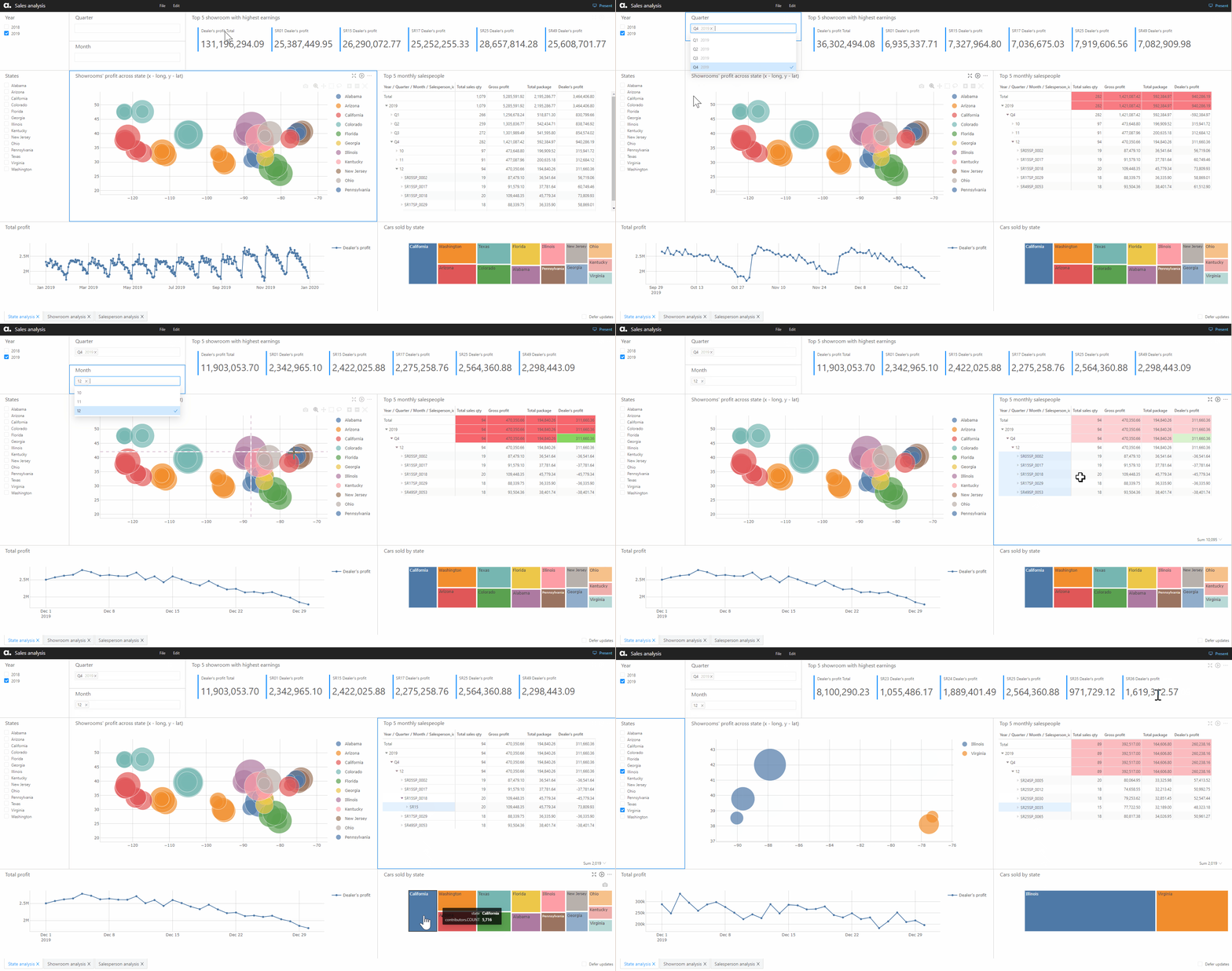
Atoti comes with its own web application where users can easily build dashboards on top of the multidimensional cube.

Aside from the profit and number of cars sold by the dealership at the state level, we are able to see the top 5 showrooms with the highest earnings globally. Likewise, we also see the top 5 salespeople for each month, along with their pay package and the number of cars they sold for the month.
Using page filters on the Atoti dashboard, we can interactively toggle the page to display the sales over the year or drill down to the month. Similarly, we can also filter the page by state.
On the page below, we split the profit chart by showroom, to show the profit trend at the showroom level for the selected states.
In the event business management has a question that is not available on the dashboard, we can easily make modifications on the spot.
Showroom-level analysis
Using radio buttons for the page filter on state, we force the page to be display statistics for a single state each time. This allows us to access the showrooms within the selected state.

The first thing we observe on the above page is that the number of cars sold is not equivalent to the profit. Showroom SR01 has the highest profit but it sold lesser cars than SR00. SR01 also has a higher percentage payout to the salespeople compared to SR00.
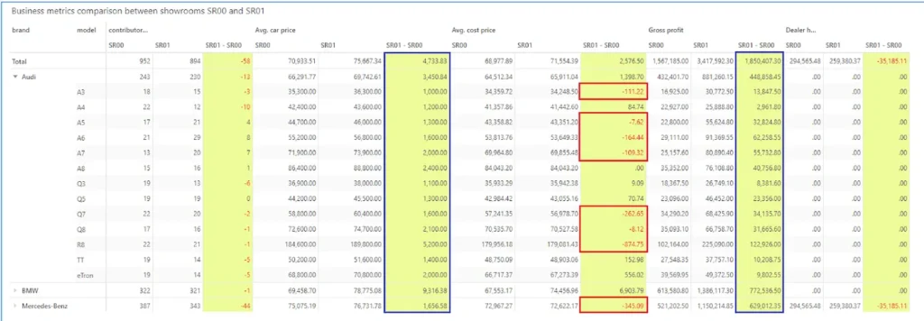
We can display the difference in the business metrics between the two showrooms using the KPI widget as shown above.
Showroom SR01 generally set a higher selling price for their cars than SR00 and their cost price is lower. Hence, their gross profit is also higher than SR00. Maybe showroom SR00 can readjust their pricing strategy to bring up their profit margin.
Salesperson analysis
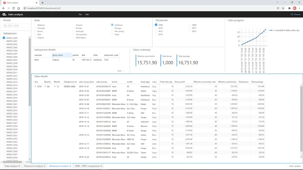
In the Salesperson dashboard view, we can dive into the sales of a single person to see the details of his sales.
Not all questions answered? Download the notebook and have a try! ⊂(▀¯▀⊂ )
Let’s understand a little more about how the commission structure works in our use case. Then, we will see how we arrived at our solution.
Commission structure in car sales
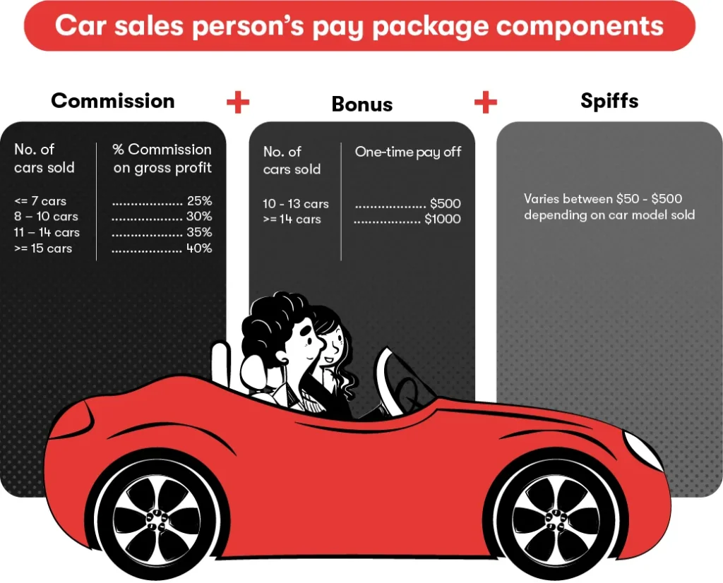
Some salespeople are given a base salary equivalent to the minimum wage. Mostly, the bulk of their pay comes from the sales commissions, a bonus if they hit a certain sales target or spiff for certain cars.
In our use case, we will assume the pay package of a salesperson to be computed as follows:
Sales data extension
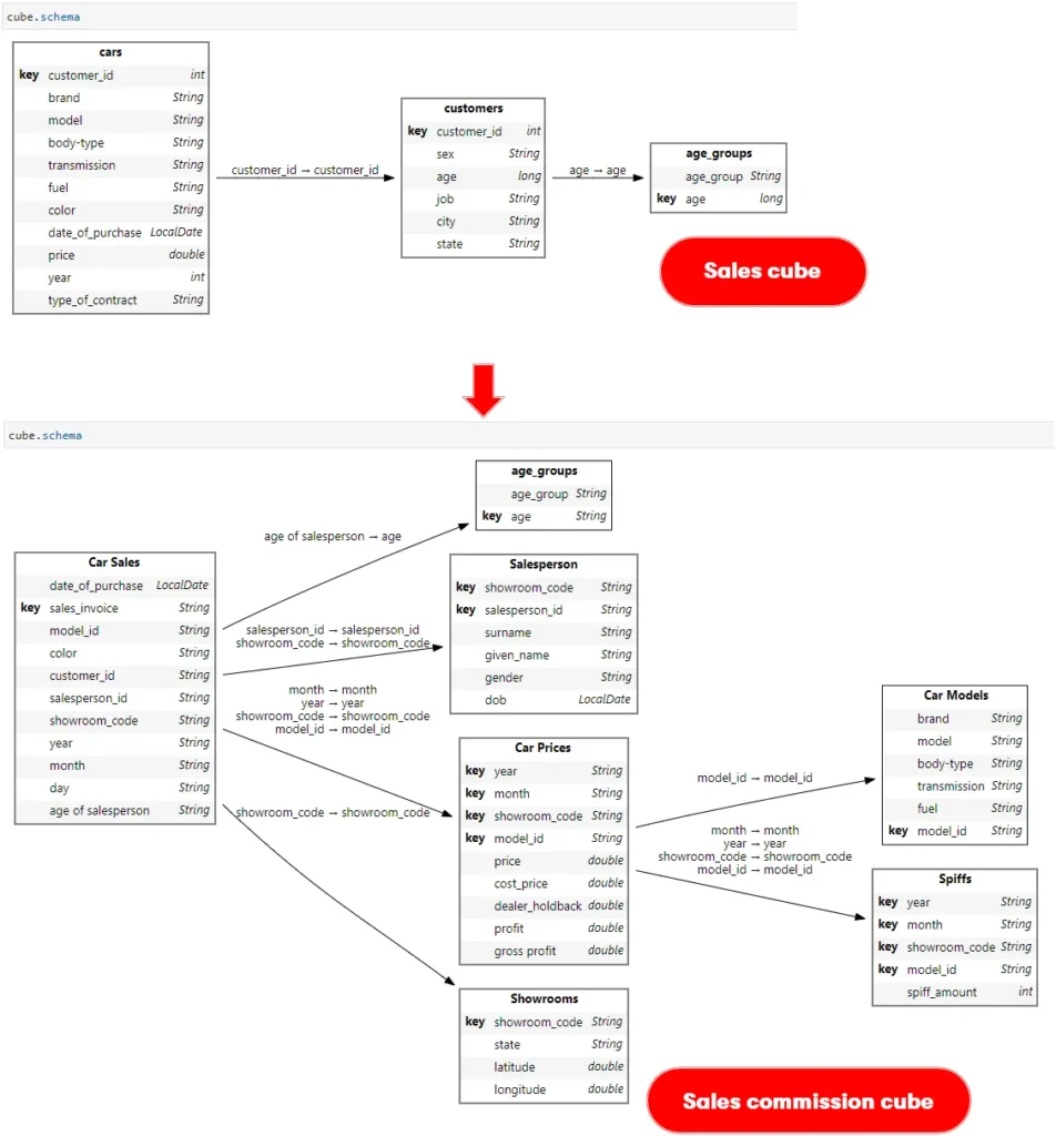
In order to achieve our objective of deriving commission for the salespeople, we extended the sale cube’s data model to include data for:
- Showrooms
- Salesperson
- Car prices by showrooms
- Spiffs for car models
We also refactored existing tables by extracting the car details into a separate table – Car Models.
Understanding how measures work in a cube
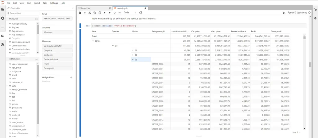
Atoti usually automatically creates measures for numerical columns in the base table when a cube is created in auto mode. Our base table-Car Sales in this case- has no numerical values. Therefore, we only have the default measure-contributors.COUNT– which shows the number of contributing facts.
DO NOT belittle this one little measure. In our use case context,
contributors.COUNTis the number of cars sold!
As we can see below, depending on the hierarchies added to the pivot table, we can get the total number of cars sold across all the dealerships, by a salesperson in total or broken down into year, month or even date.
Creating measures from referenced tables
To query the numerical values from referenced tables such as the Car Prices or Showrooms tables, we need to create measures for them.
Sum measures from table columns
m["Car price"] = tt.agg.sum(car_pricing["price"])
m["Cost price"] = tt.agg.sum(car_pricing["cost_price"])
m["Dealer holdback"] = tt.agg.sum(car_pricing["dealer_holdback"])
m["Profit"] = tt.agg.sum(car_pricing["profit"])
m["Gross profit"] = tt.agg.sum(car_pricing["gross profit"])
m["Total spiff"] = tt.agg.sum(spiffs["spiff_amount"])
Mean measures from table columns
m["Avg. car price"] = tt.agg.mean(car_pricing["price"])
m["Avg. cost price"] = tt.agg.mean(car_pricing["cost_price"])
Value as it is from the table columns
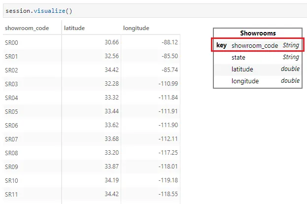
Longitude and latitude are unique values for each showroom. Therefore, we can use Atoti.value on the table column.
m["latitude"] = tt.value(showroom["latitude"])
m["longitude"] = tt.value(showroom["longitude"])
We are able to query these new measures (except for longitude and latitude) along any hierarchy and its value gets computed on the fly.
When using Atoti.value as in the case of longitude and latitude, the measure has to be queried along with the key of the table in order to return results.
Creating measures to compute commission
It is easy to compute commission. We simply take the final sales quantity by the salesperson to get the effective commission rate and multiply it by the total gross profit.
What would be interesting is how we want to track the commission?
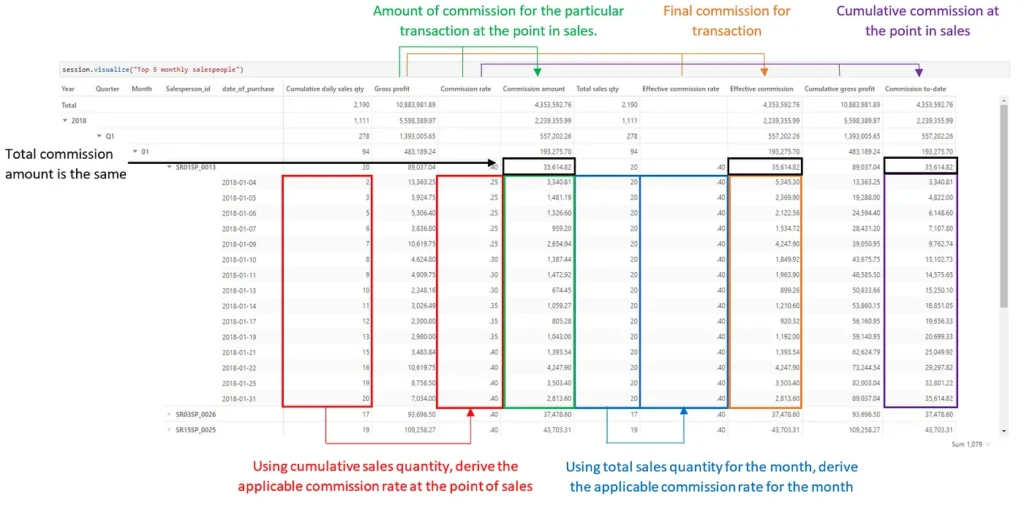
In the pivot table above, we have three different measures for commission:
- Commission amount
- Effective commission
- Commission to-date
The total commission computed for these 3 measures for the salesperson is the same. The difference lies in what we see in the drill-down. Let’s take a look at their definitions:
m["Commission amount"] = tt.agg.sum(
    m["Commission rate"] * m["Gross profit"], scope=tt.scope.origin(l["Salesperson_id"])
)

m["Commission to-date"] = tt.agg.sum(
    m["Commission rate"] * m["Cumulative gross profit"],
    scope=tt.scope.origin(l["Salesperson_id"]),
)

m["Effective commission"] = tt.agg.sum(
    m["Effective commission rate"] * m["Gross profit"],
    scope=tt.scope.origin(l["Salesperson_id"]),
)
Both Commission amount and Commission to-date uses the same commission rate in the computation. It shows the commission at the point in sales. The difference, however, is that Commission to-date uses the cumulative gross profit, hence it gives the total commission earned up to the point in sales.
On the other hand, Commission amount shows the commission of the transaction itself at that point in time. Hence, Commission to-date would be more informative as it shows the actual commission earned to date.
Effective commission is computed based on the commission applicable at the point of querying, i.e. based on the total sales volume when queried. Therefore, we can sum up the Effective commission for each transaction to get the total commission. This is different from Commission to-date, where the amount at the transaction level shows the total commission at that point in time. Hence, the last transaction of the month will reflect the total commission earned.
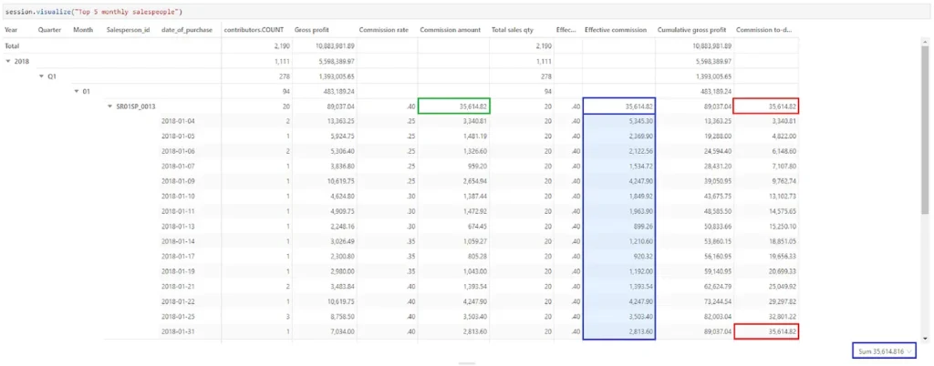
Which measure is better? It depends on the type of questions we want to answer to business.
Next, let’s look at how we create the cumulative sales quantity and gross profits, as well as the effective commission rate that is being used.
Creating cumulative measures
Using the Atoti cumulative scope, we can accumulate the value of a measure with the scope of a date level. In the case below, we accumulate the contributors.COUNT and Gross profit to get the cumulative sales quantity and cumulative gross profit respectively with the date of purchase.
m["Cumulative daily sales qty"] = tt.agg.sum(
    m["contributors.COUNT"], scope=tt.scope.cumulative(l["date_of_purchase"])
)

m["Cumulative gross profit"] = tt.agg.sum(
    m["Gross profit"],
    scope=tt.scope.cumulative(l["date_of_purchase"]),
)
We can also use the cumulative scope to create rolling windows. Check out the documentation.
Computing effective commission conditionally
Using atoti.where function, we can set the value of a measure conditionally.
m["Effective commission rate"] = tt.where(
    l["Salesperson_id"] != None,
    tt.where(
        m["Total sales qty"] <= 7,
        0.25,
        tt.where(
            m["Total sales qty"] <= 10,
            0.3,
            tt.where(m["Total sales qty"] <= 14, 0.35, 0.4),
        ),
    ),
)
We can embed where conditions embedded in existing where conditions as shown above.
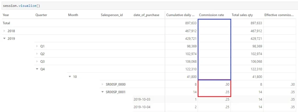
In the case of commission rate, it is pointless to aggregate the commission rate across all the salespeople as the final commission rate will not give us the total commission paid to all the salespeople. In this case, we see the condition l["Salesperson_id"] != None preventing levels above the Salesperson_id (highlighted in blue below) from having a commission rate value.
Computing one-time bonus payout
Salespeople who hit their sales targets for the month receive a one-time bonus. Here, we have the option of using the Total sales qty or Cumulative daily sales qty to see the amount of bonus the salesperson is entitled to.
Which measure to use? Again, it boils down to what we want to see in the drill-down.
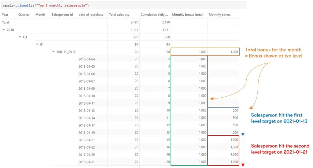
Notice that the total bonus for the month is not a sum of its underlying values? We have not performed any aggregation but instead, derived conditionally based on the sales quantity at the subtotal level of Salesperson_id.
Using Cumulative daily sales qty would be more informative in this case, as it shows us when the bonus is applicable and how much is to be given out at the point in time.
m["Monthly bonus"] = tt.where(
    l["Salesperson_id"] != None,
    tt.where(
        m["Cumulative daily sales qty"] >= 14,
        1000,
        tt.where(m["Cumulative daily sales qty"] >= 10, 500),
    ),
)
Deriving total pay package for a salesperson
We know the salesperson’s pay package comprises of three components:
- Commission
- Bonus
- Spiffs
So, simply sum them up:
m["Total bonus"] = tt.agg.sum(
    m["Monthly bonus"], scope=tt.scope.origin(l["Salesperson_id"])
)

m["Total package"] = tt.agg.sum(
    m["Effective commission"] + m["Monthly bonus"] + m["Total spiff"],
    scope=tt.scope.origin(l["Salesperson_id"]),
)
We performed an aggregation on the Monthly bonus so that we can get its corresponding value above the Salesperson_id level.
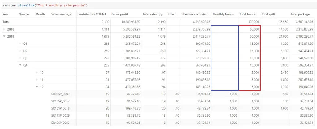
Atoti.agg.sum sums up the value of the underlying level to give a sub-total at the current levelNow we can understand the pay package of a salesperson down to the transaction level.
Getting Dealer’s profit
What’s the profit for the dealers after paying the salespeople?
m["Dealer's profit"] = m["Profit"] - m["Total package"]We used Profit instead of Gross Profit here because dealers earn the dealer’s holdback, which is not included in the gross profit.
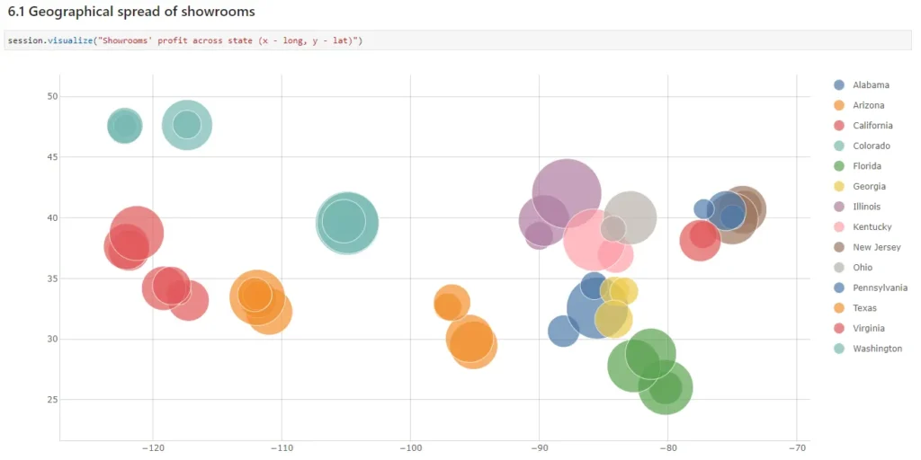
Putting it all together, we can now see the spread of the showrooms geographically, with its size represented by its profit.
Want more..?
Continue to explore different aspects such as the performance of salespeople by their age group or gender to see if it makes any difference. You can also use the parameter simulation to adjust the commission rates to see the downstream impacts!
Download the notebook and have some fun!
