Building regulatory risk application with Python and Atoti
In this post, I want to discuss a faster approach to compute the variance-covariance formulas present in financial regulatory capital models – FRTB SBM and CVA Risk Framework – as well as ISDA SIMM and internal sensitivity-based VaR-type models, and illustrate this approach with a sample implementation of SBM Equity Delta aggregation in Atoti. I would like to thank Robert Mouat for sharing his research on the matrix formula optimization and multi-threading in the FRTB Accelerator.
All of the above-mentioned methodologies use a series of nested variance-covariance formulae – see an example below – to compute a VaR-like risk measure. For the justification of the nested variance-covariance formulas please refer to “From Principles to Model Specification” document by ISDA SIMM, March 3, 2016.
One of the roll-up steps involves a high-cardinality operation – aggregating risk factors into buckets – since there might be thousands of risk factors in certain risk classes, for instance, in credit spreads and equities, brute-force application of the formula is expensive. Since we want to be able to recompute SBM dynamically, explore portfolios and apply simulations, the efficiency of the calculation is critical.
The naïve approach to the bucket-level aggregation has O(N2) time complexity:

The trick is to leverage the fact that many of the risk factor pairs use the same value of the correlation 𝞺kl – so that it can be taken out of the double sum and the formulae can be rearranged.
Equity Delta Bucket-Level Rollup Optimisation
We’ll group the pairs of equity delta risk factors sharing the same correlation value. The Equity Delta risk factor correlations are set in paragraph [MAR21.78] of the Consolidated Basel Framework and allow us to break the pairs as follows:
- Group 1: same name, different type (spot/repo): constant value 0.999 per MAR21.78
- Group 2: different name, same type: a single value depending on the bucket, for example, 0.15
- Group 3: different name, different type: value depending on the bucket and multiplied by 0.999, for example, 0.15 x 0.999
Now let’s look at how the formulae can be rearranged for groups of risk factor pairs having the same risk factor correlation.
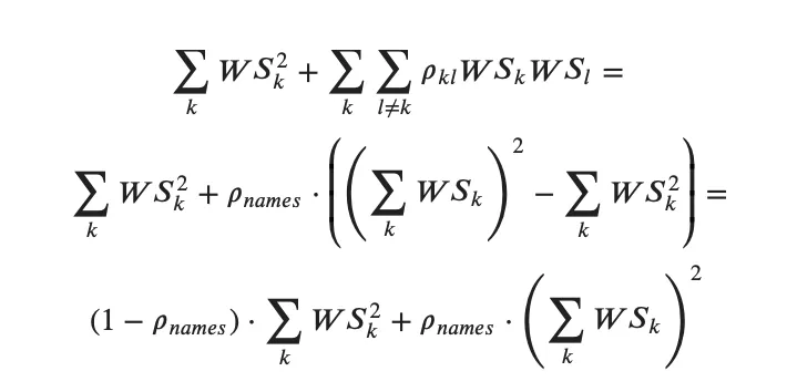
Let’s start with the pairs where both risk factors are either spot or repo – cases 1. and 2. above. Since for any 𝑘 and 𝑙 the correlation 𝜌𝑘𝑙 will be equal to the correlation defined per bucket 𝜌𝑛𝑎𝑚𝑒𝑠, their contribution can be rewritten – “reduced formula”:

This calculation is O(N) complexity.
Python implementation
I used python and Atoti to implement this formula as follows:
# This measure will display the sum of WS_k squared by risk factor (Qualifier + Label2):
m["sum squares"] = tt.agg.square_sum(
    m["WS"], scope=tt.scope.origin("Qualifier", "Label2")
)
reduced_formula = (1 - m["names_correlation.VALUE"]) * m["sum squares"] + m[
    "names_correlation.VALUE"
] * tt.pow(m["WS"], 2.0)

# Total contribution:
# - of the pairs having only spot risk factors,
# - of the pairs having only repo risk factors,
# is the sum of the reduced formula by Label2 members.

m["spot&repo pairs contribution"] = tt.agg.sum(
    reduced_formula, scope=tt.scope.origin("Label2")
)
The contribution of the risk factors where one risk factor belongs to “SPOT” and the other belongs to “REPO” – case 3 above – can be rearranged as follows and computed with O(N) time complexity:

where:
– J – is a matrix of ones,
– first term in the above formula performs aggregation of all sensitivities as if they all are correlated at 𝜌𝑛𝑎𝑚𝑒𝑠,
– the second term is to correct the first term and to account for the fact that risk factors, where spot and repo risk factors have the same equity name, must be correlated at 0.999.
This is my code snippet implementing the contribution of pairs having spot and repo risk factors – called “cross repo spot contribution”:
# filtering for repo and spot risk factors:
m["WS_spot"] = tt.filter(m["WS"], lvl["Label2"] == "SPOT")
m["WS_repo"] = tt.filter(m["WS"], lvl["Label2"] == "REPO")

# Collect WS of the spot risk factors in a vector and show against every qualifier in a bucket:
m["weights_vector"] = tt.agg._vector(
    m["WS_spot"], scope=tt.scope.origin(lvl["Bucket"], lvl["Qualifier"])
)

m["spot vector"] = tt.total(m["weights_vector"], h["Qualifier"])

# cross product of weighted sensitivities for the names, having both spot and repo sensitivities:
# Multiply vector WS of the spot risk factors by WS of each repo risk factor sum them up
repo_scalar_x_spot_vector = m["WS_repo"] * m["spot vector"]
m["sum WS_repo |J| WS_spot"] = tt.agg.stop(
    tt.agg.sum(
        tt.array.sum(repo_scalar_x_spot_vector),
        scope=tt.scope.origin(lvl["Bucket"], lvl["Qualifier"]),
    ),
    lvl["Bucket"],
)
m["WS_spot_parent"] = tt.agg.sum(m["WS_spot"], scope=tt.scope.origin(lvl["Label2"]))
m["WS_repo_parent"] = tt.agg.sum(m["WS_repo"], scope=tt.scope.origin(lvl["Label2"]))


m["sum WS repo and spot"] = tt.agg.stop(
    tt.agg.sum(
        m["WS_spot_parent"] * m["WS_repo_parent"],
        scope=tt.scope.origin(lvl["Qualifier"]),
    ),
    lvl["Bucket"],
)
# final contribution of the pairs where one risk factor is spot, one is repo
m["cross repo spot contribution"] = (
    m["names_correlation.VALUE"] * m["sum WS_repo |J| WS_spot"] * 0.999
    + 0.999 * (1 - m["names_correlation.VALUE"]) * m["sum WS repo and spot"]
)
Combining the spot, repo and cross spot/repo paris into Kb measure and checking whether the bucket is 11 or not (see Kb formula for bucket 11 in [MAR21.79]):
m["Kb"] = tt.where(
    lvl["Bucket"] == "11",
    tt.agg.sum(tt.abs(m["WSk"]), tt.scope.origin("Qualifier", "Label2")),
    tt.sqrt(
        tt.max(
            0, m["spot&repo pairs contribution"] + 2 * m["cross repo spot contribution"]
        )
    ),
)
Dynamic aggregation in Atoti
I used the above rearranged formulas to implement measures for the on-the-fly aggregation with python and Atoti, you can download my example here: Notebook example for Equity Delta SBM.
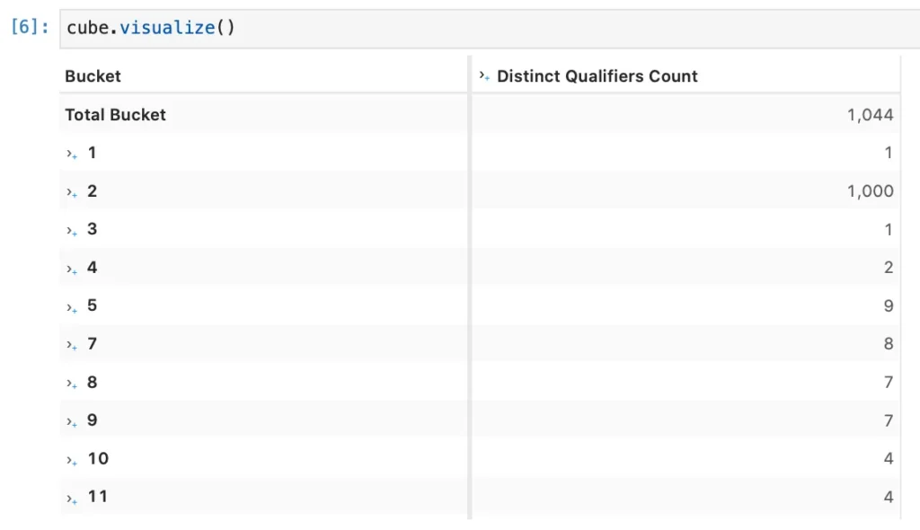
My sample data has about 1000 different names, and most of them sit in bucket #2,

and the whole SBM chain from sensitivities to weighted sensitivities to bucket level charges and equity delta risk charge is re-aggregated interactively:
Let’s look at how the chain of SBM measures can be implemented.
I’m using Atoti where function to check whether I should use the basic or formula for the Delta margin as prescribed in [MAR21.4(5)(b)(ii)]:
m["Delta Charge"] = tt.where(
    m["sum Kb2 + sum sum WSb WSc gamma"] > 0,
    tt.sqrt(m["sum Kb2 + sum sum WSb WSc gamma"]),
    tt.sqrt(m["sum Kb2 + sum sum Sb Sc gamma"]),
)
When Sb is equal to the net weighted sensitivity – as per the basic formula in MAR21.4(5)(a) – I’m using square_sum and sum aggregation functions in Atoti:
m["sum Kb2 + sum sum WSb WSc gamma"] = tt.agg.square_sum(
    m["Kb"], scope=tt.scope.origin("Bucket")
) + tt.agg.sum(
    m["WSb"] * m["WSc"] * m["gamma.VALUE"], tt.scope.origin("Bucket", "Other Bucket")
)
To implement the alternative formula from [MAR21.4(5)(b)], I’m first computing the Sb and Sc and then aggregating them.
m["Sb"] = tt.max(
    tt.min(m["WSk"], m["Kb"]), -1.0 * m["Kb"]
)
m["Sc"] = tt.at(m["Sb"], {lvl["Bucket"]: lvl["Other Bucket"]})
m["sum Kb2 + sum sum Sb Sc gamma"] = tt.agg.square_sum(
    m["Kb"], scope=tt.scope.origin("Bucket")
) + tt.agg.sum(
    m["Sb"] * m["Sc"] * m["gamma.VALUE"],
    scope=tt.scope.origin("Bucket", "Other Bucket"),
)
We’ve discussed the bucket-level calculation – “Kb” – in details in the previous section, so the only measure that we haven’t discussed so far is the weighted sensitivity calculation which is trivial:
# The input sensitivities are multiplied by the risk weight for each Bucket and Label2,
# and then summed up to obtain weighted sensitivities:
m["WS"] = tt.agg.sum(
    m["AmountUSD.SUM"] * m["RW.VALUE"], scope=tt.scope.origin("Bucket", "Label2")
)
Please refer to the notebook example if you wish to learn more about input data and model that I used.
Conclusion
In this post, we discussed how to rearrange the variance-covariance formula so that it can be computed more efficiently. Two additional notes on that:
- We looked at the equity delta example and a certain way to rearrange the formula – there exists a way to rearrange the formula consistently across sensitivity types and risk classes
- In the FRTB SBM methodology, many of the correlations are defined as single values set per bucket. Although similar, the SIMM calculations are a bit harder to optimize as high concentrations may trigger adjusted correlation values for some of the risk factor pairs. However if for most of the netting sets/risk factors the exposures are below the concentrations, the algorithm will still be close to linear time.


