
Atoti is a Python library that allows us to easily create an operational intelligence platform. Users can analyze and visualize complex data in a collaborative and scalable environment. Atoti’s in-memory solution facilitates quick processing speeds and dramatically accelerates query performance. With the use of aggregate providers, we can go even further to speed up our queries and ultimately save time and resources.
What are aggregate providers?
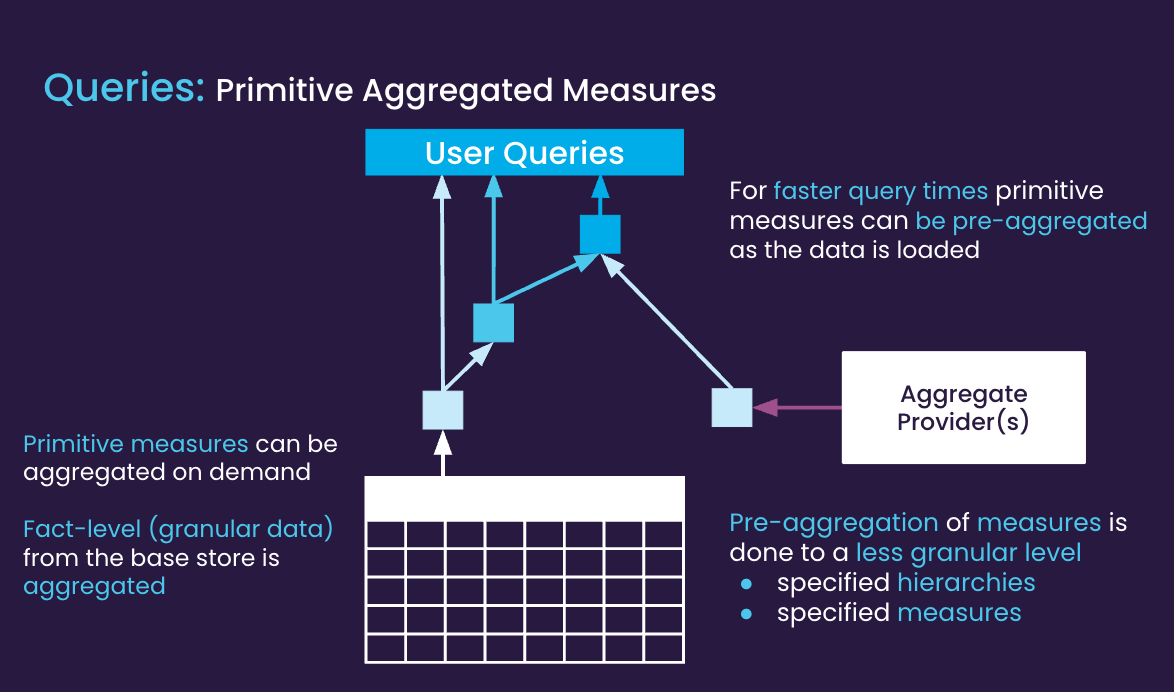
Primitive aggregated measures are created from raw data in the database when a user queries Atoti. These aggregated measures can then combine to compute other intermediate or top-level measures. An aggregate provider speeds up query time by storing primitive or intermediate aggregates in-memory and avoiding queries to the fact table directly. Hierarchies and their levels determine the scope and depth of the pre-aggregation.
For instance, given the following cube schema:
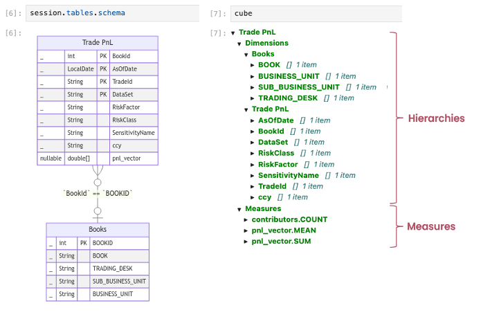
We can create an aggregate provider that helps to speed up the query of the measure pnl_vector.SUM when queried across selected levels for the current reporting date:
cube.aggregate_providers.update(
    {
        "PnL provider": tt.AggregateProvider(
            key="bitmap",
            levels=[
                l["AsOfDate"],
                l["BUSINESS_UNIT"],
                l["SUB_BUSINESS_UNIT"],
                l["TRADING_DESK"],
            ],
            measures=[m["pnl_vector.SUM"]],
            filter=(l["AsOfDate"] == current_date),
        )
    }
)
On a local instance where the data is loaded in-memory, the query time reduces by more than half with the aggregate provider:
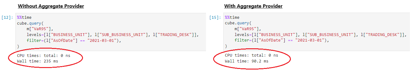
The savings become more obvious when we connect to a cloud data warehouse. We can see that the query time goes from seconds to milliseconds.
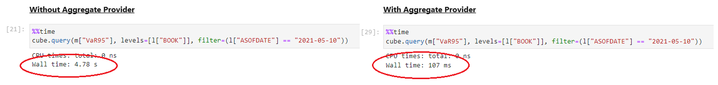
We see that the query time reduces from close to 5 seconds to 107 milliseconds. This is because the aggregate provider stores the aggregated results in-memory. Hence, we save from not having to query the cloud database again. Less queries to the cloud means more saving on cost!
💡 Note: CPU Time measures the actual time the processor spends executing a task, excluding waiting for I/O, network, or other processes. Wall Time is the total real-world time from the start to the end of execution, including delays like I/O, network latency, and waiting for other processes.
Understanding aggregate providers
Let’s try to understand the aggregate provider through the different parameters of the function, for example:
tt.AggregateProvider(
    key="bitmap",
    levels=[
        l["AsOfDate"],
        l["BUSINESS_UNIT"],
        l["SUB_BUSINESS_UNIT"],
        l["TRADING_DESK"],
    ],
    measures=[m["pnl_vector.SUM"]],
    filter=(l["AsOfDate"] == current_date),
    partitioning="modulo4(trades_tbl.AsOfDate)"
)
1. Key
By default, Atoti uses the JUST IN TIME (JIT) aggregate provider to retrieve its aggregates directly from the database as required during runtime. There is no pre-computation of aggregates, therefore queries are slower. Its performance greatly depends on the optimization in the tables, e.g. partitioning etc.
However, with the aggregate provider function, we can define different types of aggregate providers to help speed up specific queries.
There are two types of aggregate providers for the function:
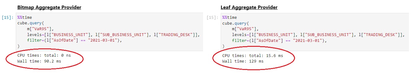
- leaf: Leaf aggregate provider
The leaf aggregate provider retrieves pre-computed aggregates using a point index. The point index lists all the locations in the cube for the given hierarchies. The aggregate provider uses the index to retrieve pre-aggregations from these locations. The leaf aggregate provider’s performance is significantly greater than that of the JIT aggregate provider. However, it has a higher memory cost than the JIT aggregate provider due to the point index.
- bitmap: Bitmap aggregate provider
The Bitmap aggregate provider is a leaf aggregate provider that uses a point index, but also a bitmap index to more quickly retrieve pre-computed aggregates at query time. The bitmap aggregate provider resolves filtering conditions more quickly than the leaf aggregate provider. As a result, the bitmap aggregate provider is faster than the leaf aggregate provider, but also uses more memory.
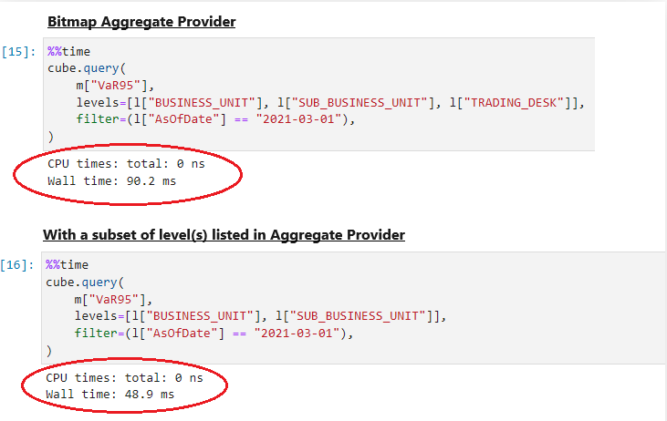
2. Levels
We use the levels parameter to define the levels to build the provider on:
- AsOfDate
- BUSINESS_UNIT
- SUB_BUSINESS_UNIT
- TRADING_DESK
A JIT provider is often used when querying data directly from the fact table, but depending on the levels we defined for each of our providers, we may be using a mix of several providers in our queries. We call these “partial” aggregate providers. Atoti decides on the most appropriate way to retrieve the aggregate at query time, depending on the query measures and locations. This helps to achieve the appropriate trade-off between memory consumption and query performance.
Let’s see how some of the queries behave with the use of the aggregate provider we have defined. As we query levels along any combination of these levels, we can see the performance improves.
We can also use the explain parameter of cube.query to understand what type of providers are used in the retrieval:
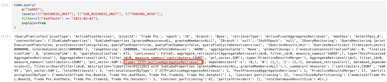
Before Aggregate Provider
Before implementing an aggregate provider, the query plan shows that we use the JITPrimitiveAggregatesRetrieval to retrieve our query:
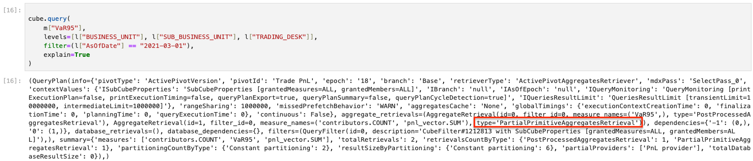
After aggregate provider
After implementing an aggregate provider, the query explain plan shows that we are now using the PartialPrimitiveAggregatesRetrieval to retrieve our query.
Despite defining an aggregate provider, we should be mindful of how we are expecting aggregate providers to speed up our queries. There are instances when querying the database may not use an existing aggregate provider:
- A level expressed in the query belongs to a level that is not part of the definition of the aggregate provider.
- A level expressed in the query is deeper than the level defined for the aggregate provider.
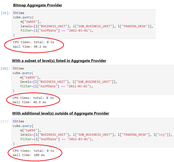
For example, the level ccy is not defined in the aggregate provider. When using the ccy level in our query, the JIT aggregate provider is used to query the fact-level data instead of the pre-aggregates stored in-memory:

Using aggregate providers to speed up queries comes with a cost in terms of memory. Therefore we must be selective about what we store in memory by investigating the type of queries that are most frequent. It may be more useful to define partial providers that cover subsets of hierarchies and exclude levels with high cardinalities.
3. Measures
Aggregate providers pre-compute and store in-memory the measures defined for it at specified levels. To gain the maximum benefit from using aggregate providers, we should store only the most basic measures used to build other measures.
Such basic measures are the aggregated measures derived from table fields. In our case, the pnl_vector field is the underlying fact for pnl_vector.SUM. Therefore, we pre-aggregate pnl_vector.SUM in our aggregate provider.
When we look at the measure VaR95, it is built on top of the existing measure pnl_vector.SUM in its definition:
m["VaR95"] = tt.array.quantile(m["pnl_vector.SUM"], 1 - 0.95)Although VaR95 is not defined in our aggregate provider, we can see the performance of the query for the measure improve dramatically with the use of aggregate providers. This is because VaR95 aggregates on top of pnl_vector.SUM, which is already available in-memory due to the aggregate provider defined for it.
💡 Note: In general, deciding to add one more measure to an existing aggregate provider will not greatly increase the memory footprint of the provider, unless this measure computes vectors.
4. Filter
When dealing with a large volume of data, we can add filters to a partial aggregate provider to pre-aggregate for a matching subset of data. This reduces the memory cost of the aggregate provider. To do so, we make use of the filter parameter to set the condition(s) for the data used for pre-computations.
We can have a combination of conditions for our filter but it is important to know that the filter works only on equality tests on levels. I.e. we cannot have a range comparison or a comparison on the value of measures.
A combination of conditions may look like this, with the use of the & or | operator for AND and OR operations:
filter=(l["AsOfDate"] == current_date) & (l["BUSINESS_UNIT"] == "Equity")5. Partitioning
Partitioning a table is to organize the data that the table holds and separate them into different pieces or partitions. This distributes the work performed by the processing cores for both data loading and querying.
When setting the partitioning for aggregate providers, it is useful to know that the default setting is to use the partitioning of the cube’s fact table. However, we can also specify a particular method of partitioning. This may be useful when a particular partitioning method works best when querying data as opposed to loading data in the database:
partitioning="modulo4(trades_tbl.AsOfDate)"To explore this topic further, reach out to the Atoti team on GitHub discussion.
Give it a try
Check out the notebook on Aggregate Provider in Atoti GitHub. Or, if you have an interest in how aggregate providers can speed up querying for cloud databases, check out the notebook Atoti DirectQuery with Snowflake.