A case study on better retail pricing based on location-based competitors’ price data through Machine Learning
Retailers are relying more and more on technology to optimize their pricing strategies to maintain or improve their sales and bottom line. Deploying those strategies has become increasingly profitable – and necessary to stay competitive – with the widespread availability of a variety of data, such as competitor prices.
In this article, we will see how a retailer can group their shops into sets based on the geographical distribution of competitors and apply different price strategies based on the characteristics of each cluster. Machine learning helps us identify the clusters of shops and we use Atoti to analyze the characteristics of each cluster and optimize pricing.
This will provide a good example of using Atoti to exploit the results of machine learning algorithms,
Quick links to sections:
Interpreting machine learning results with Atoti
Our imaginary use case
Imagine a retailer in France with shops spread across the country. Each shop is shown as a red pin in the map below.
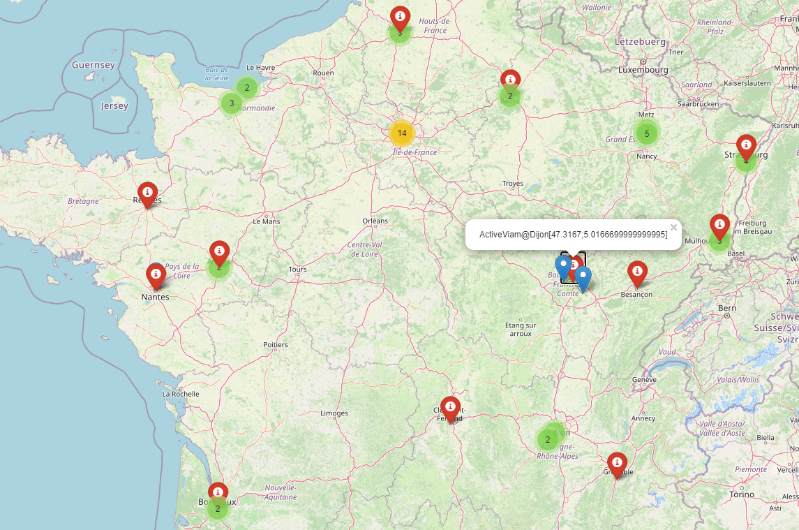
The competitor outlets are shown as colored dots and blue pins on the map.
Every shop performs differently. For the purpose of optimization, it is necessary to identify a pattern in their environment and competitive strengths to explain this difference in performance.
What data do we have?
We have geographical information for each of our shops and for our competitors’. Using haversine formula on the latitude and longitude of the shops, we determined the distance between each retail shop and all its competitors.
We also have data on the products and their sales figures for each shop as well as the local competitors’ selling price of the same products.
Objective
To identify the clusters of shops, we need to prepare the feature inputs of each shop for machine learning:
- The number of competitors by distance buckets of e.g. 1km, 5km, 10km, etc.
- Price index – our price position against competitors
Once we have our clusters output from machine learning, we will optimize prices using a pricing engine and analyze the impact using Atoti.
Number of competitors per distance bucket
Every one of our shops has a different number of competitors within its region. With Atoti visualization, we see the number of competitors within different distance buckets from each shop.
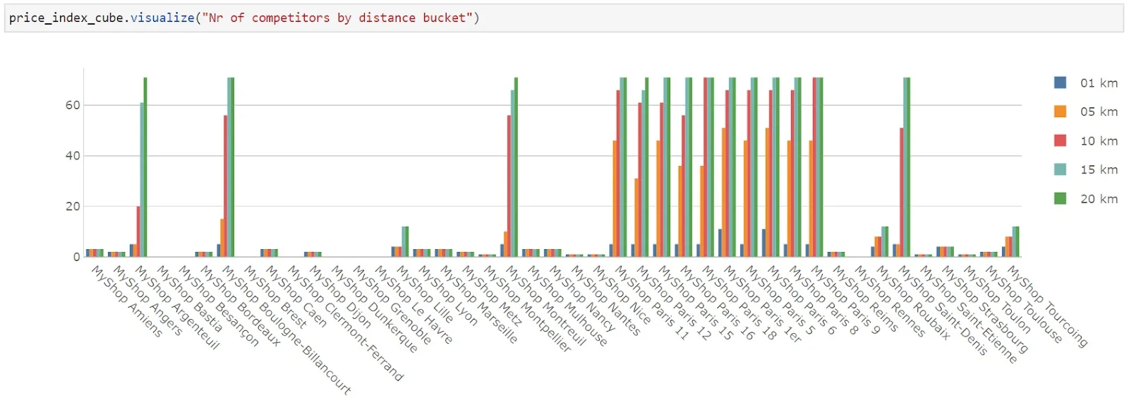
From the clustered column chart above, we see that shops in Montpellier, Nantes, Nice, Saint-Etienne, etc. have very little competition within a 20km distance radius. If we look at the shops around Paris, for instance, MyShop Paris 11, 12, 15, we see that while there are few competitors within 1km, a lot of competitors are located within a 5km radius.
Price Index
The price index is a measurement of where a retailer is positioned compared to one or several competitors.
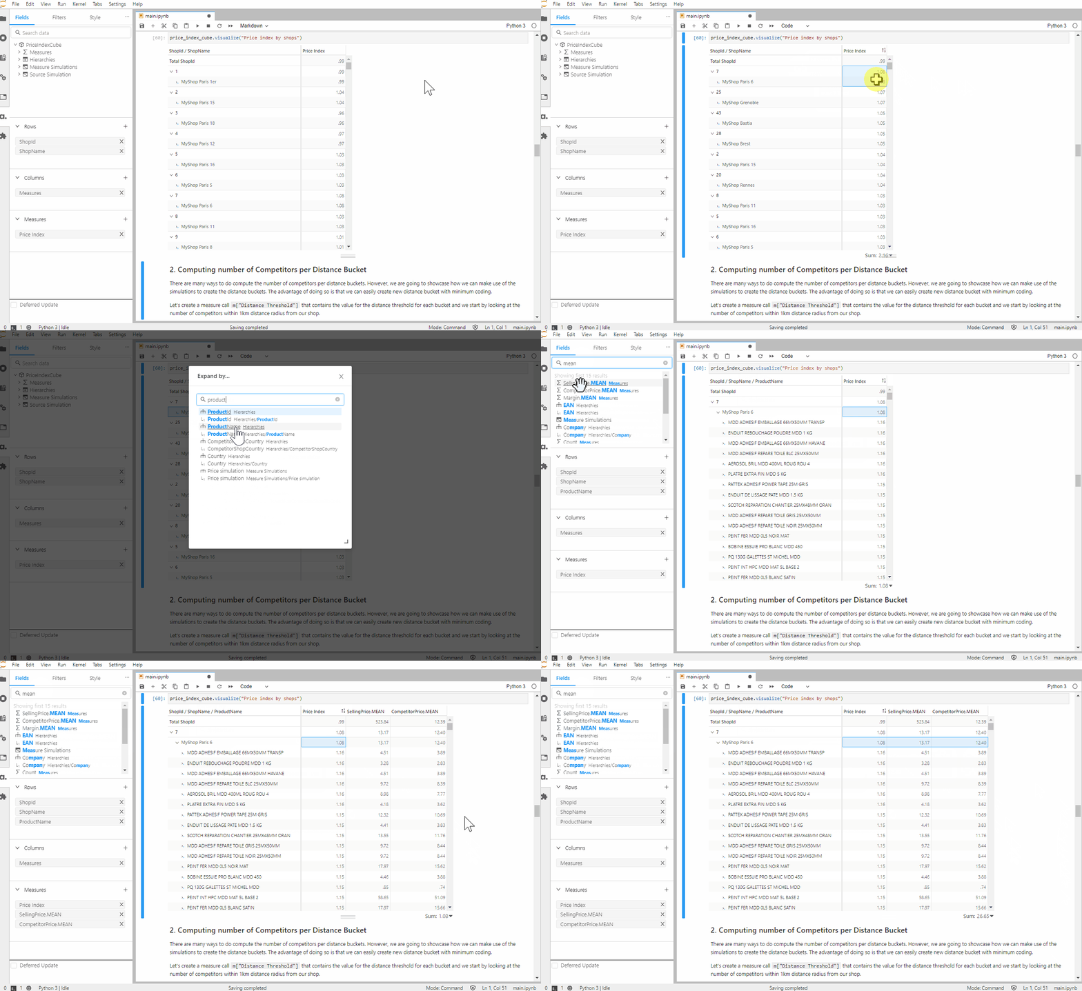
When we look at the price index, a value of 1.00 indicates that the selling price of the product in our shop is the same as the average selling price of our competitors. A value greater than 1 shows that we are selling at a higher price. Similarly, a value lower than 1 shows that we are selling at a lower price than most of our competitors.
We could adjust the selling price of each product, or clusters of products, as we have demonstrated in a different article – Data dive: How to improve pricing strategies with a set of checkout receipts. However, in this article, we adjust the selling price for our shops such that if there is high competition, we lower the price index. If there is low competition, we can afford to have similar or higher selling prices.
Implementation
We will skip the implementation of the Atoti datacube as we focus more on the machine learning and data analytics aspect here.
Data Schema
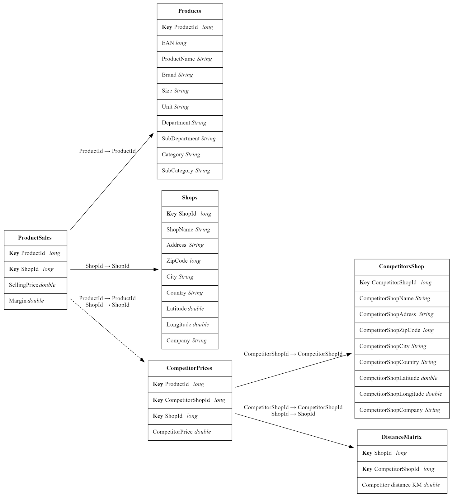
We have the resulting snowflake schema:
Measure computation
Computing the number of competitors per distance bucket
While there are many ways to compute the number of distance buckets, we wanted to showcase how we can do so with Atoti’s scenario feature. If we set the distance radius from the shop as a threshold, the scenario feature allows us to run simulations with different values for the distance radius, hence achieving the distance bucket.
For instance, we start by looking at 1km distance radius from each shop:
m[“Distance Threshold”] = 1
We count the number of competitors who are located within the distance threshold:
m["Count within distance threshold"] = tt.agg.sum(
    tt.where(
        tt.agg.mean(m["Competitor distance KM.VALUE"]) < m["Distance Threshold"],
        1
    ),
    scope=tt.scope.origin(lvl["ShopId"], lvl["CompetitorShopId"]),
)
Did you notice here how we use the average distance between the competitors and the shop for the distance comparison? This is because the join between the CompetitorPrices and DistanceMatrix store may result in the value Competitor Distance KM to be multiplied by the number of products.

Now that we have computed the number of competitors within 1km, we set this original data as the base scenario, named as “01 km”.
simulation = price_index_cube.setup_simulation(
    "Distance Simulation", base_scenario="01 km", replace=[m["Distance Threshold"]]
)
We can now easily create as much new distance buckets as we needed, simply by replacing the distance threshold value in each scenario:
simulation.scenarios["05 km"] = 5
simulation.scenarios["10 km"] = 10
simulation.scenarios["15 km"] = 15
simulation.scenarios["20 km"] = 20
We use the cube.visualize feature to present the number of competitors in each scenario as follows:
Price Index computation
We have the following weighted price index formula:

Firstly, note that we are only interested in the relevant CompetitorPrice of competitors within a given distance threshold. We can achieve this by using the “where” condition to return the CompetitorPrice if the competitor lies within the distance threshold.
m["CompetitorPrice.MEAN"] =  tt.agg.mean(
    tt.where(m["Competitor distance KM.VALUE"] < m["Distance Threshold"], m["CompetitorPrice.VALUE"], None)
)
m["CompetitorPrice.MEAN"].formatter = "DOUBLE[#,###.00]"
Instead of using Pandas to do pre-aggregation, we perform the margin computation with Atoti so that we can see the change in its value after we optimise the selling price later on.
m["Margin.SUM"] = tt.agg.sum(
    (m["SellingPrice.SUM"] - m["PurchasePrice.SUM"]) * m["Quantity.SUM"],
    scope=tt.scope.origin(lvl["ProductId"], lvl["ShopId"]),
)
Finally, let’s see the equivalent of the above formula in Atoti.
price_index_numerator = tt.agg.sum(
    (m["SellingPrice.SUM"] * m["Margin.SUM"]) / m["CompetitorPrice.MEAN"],
    scope=tt.scope.origin(lvl["ProductId"], lvl["ShopId"]),
)
m["Price Index"] = price_index_numerator / m["Margin.SUM"]
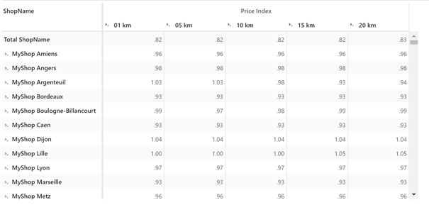
For each shop, we can see the difference in price index as the number of competitors changes with the distance threshold.
price_index_cube.visualize("price index by shops and distance")
Data output for machine learning
We can output the price index and number of competitors per distance bucket for each shop into a pandas DataFrame simply by querying the cube:
def get_features():
    # output dataframe for competitors count per shop & area (distance radius) from cube querying
    shops_competitors_count_per_shop_area = price_index_cube.query(
        m["Count within distance threshold"],
        levels=[lvl["ShopId"], lvl["Distance Simulation"]],
    ).reset_index()
    # pivot the table such that each scenario becomes a column
    shops_competitors_count_per_shop_area = shops_competitors_count_per_shop_area.pivot(
        index="ShopId",
        columns="Distance Simulation",
        values="Count within distance threshold",
    )
    # output dataframe for price index by shop from cube querying
    price_index_per_shop_area = price_index_cube.query(
        m["Price Index"], levels=[lvl["ShopId"], lvl["Distance Simulation"]]
    ).reset_index()
    # pivot the table such that each scenario becomes a column
    price_index_per_shop_area = price_index_per_shop_area.pivot(
        index="ShopId",
        columns="Distance Simulation",
        values="Price Index",
    )
    # merge the 2 dataframe and return the output
    shops_features = pd.merge(
        shops_competitors_count_per_shop_area,
        price_index_per_shop_area,
        left_on="ShopId",
        right_on="ShopId",
        how="left",
        suffixes=('', '_Price Index')
    ).fillna(1)
    return shops_features
We did 2 separate queries and merged them using pandas. In the event we have to add more distance buckets using the scenario, we simply call this function to regenerate the output for machine learning.
Machine learning
K-means clustering partitions n observations into k clusters in which each observation belongs to the cluster with the nearest mean (cluster centers), serving as a prototype of the cluster.
K-means clustering is the perfect machine learning algorithm that we needed to find groups in the data.
Let’s assume 5 clusters for retail shops and feed the below features to the algorithm:
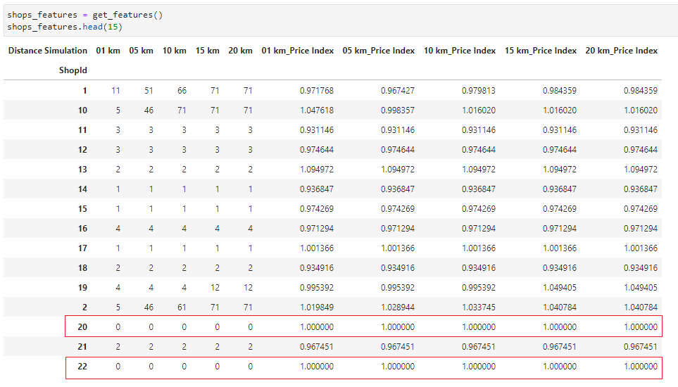
We see that the price index for ShopId 20 and 21 is 1.0. This is because the competitors of these shops are more than 20km away from them. Hence there is literally no competition nearby.
%matplotlib inline
import matplotlib.pyplot as plt
import numpy as np
import pandas as pd
import scipy as sc
import seaborn as sns
from sklearn.cluster import KMeans, MiniBatchKMeans
from sklearn.metrics import pairwise_distances_argmin
number_of_clusters = 5
kmeans = MiniBatchKMeans(number_of_clusters)
# stores_feature - dataframe containing shops and its features
kmeans.fit(shops_features)
new_colors = kmeans.cluster_centers_[kmeans.predict(shops_features)]
k_means_labels = pairwise_distances_argmin(shops_features, kmeans.cluster_centers_)
labels = KMeans(number_of_clusters, random_state=0).fit_predict(shops_features)
Using the distance bucket of 1km, let’s try to understand the output from the model:
plt.scatter(
    shops_features.loc[:, "01 km"],
    shops_features.loc[:, "Price Index"],
    c=k_means_labels,
    s=50,
    cmap="viridis",
)
plt.xlabel("Nr Competitors within 1km")
plt.ylabel("Price Index")
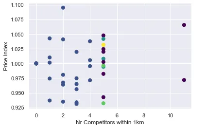
In the above plot, each color represents a cluster. We can see that clusters seem to be strongly based on the number of competitors rather than on the price index.
Let’s use seaborn to visualize the clustering results for every pair of features:
shops_features["Cluster"] = labels
sns.pairplot(data=shops_features, hue="Cluster")
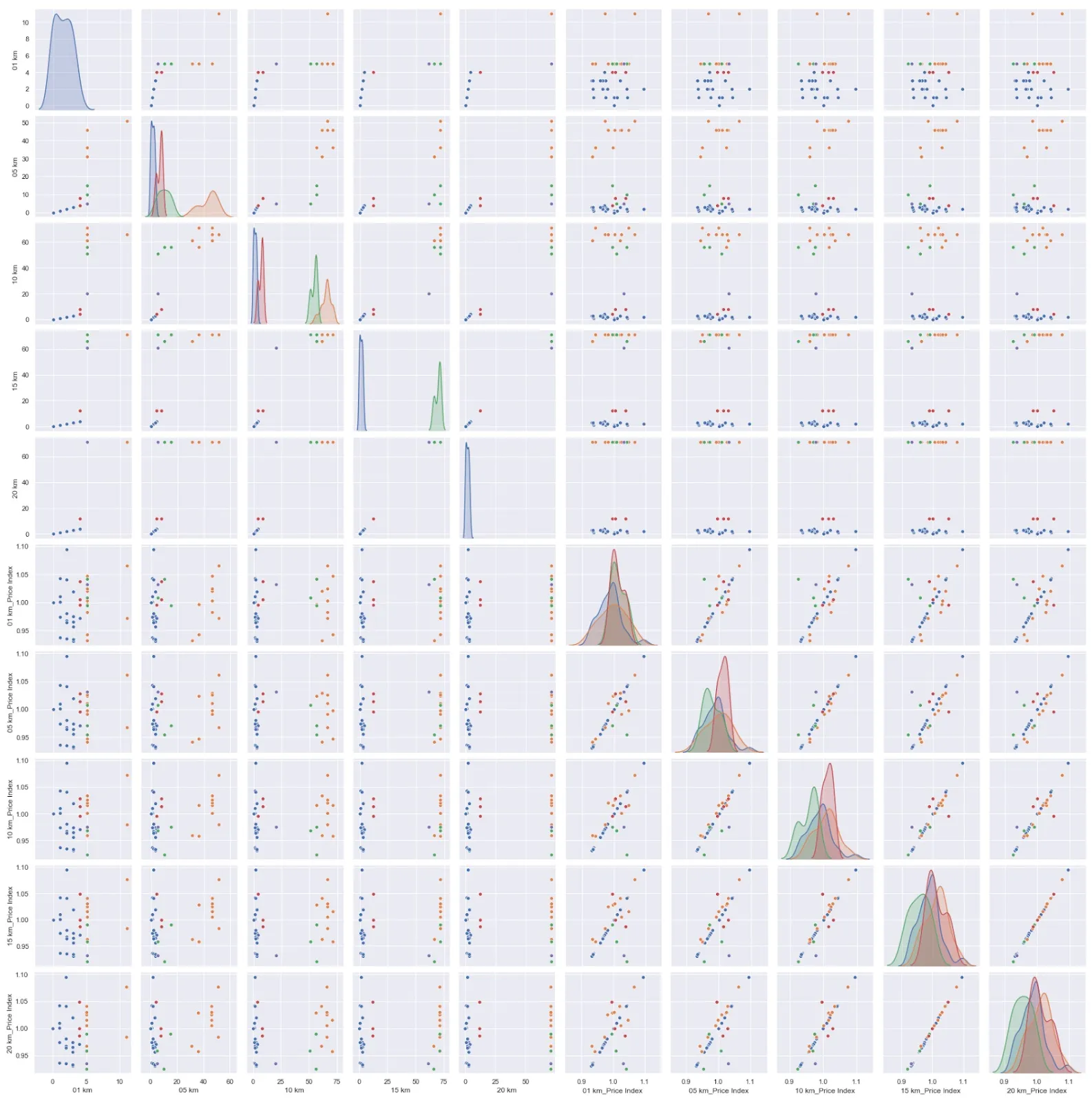
Let’s focus on the last row that depicts the relationship between the price index and the distance buckets.

The shops in cluster 1 (blue box) have a much higher number of competitors (>50) in a 10km radius, compared to those of cluster 0 (red box) having less than 20 competitors in the same radius. While cluster 1 has more competitors, its price index is generally higher than cluster 0 and greater than 1.
Continuing this analysis tells us that:
- Cluster 0 is a big cluster with few competitors around and its price index is generally around 1.
- Cluster 1 has a high number of competitors even within a 5km distance radius. However, its price index is slightly skewed towards a higher price index even with the high competition.
- Cluster 2 is a small cluster and the number of competitors increases tremendously as the distance radius increases. Generally, it has a lower price index than its competitors.
- Cluster 3 is a small cluster and the number of competitors remains about the same across all buckets. Its price index remains consistent at around 1 across the distance bucket, although one of its shops started having a higher price index and the rest fall below 1 as we consider competitors in the 15-20km radius.
- Cluster 4 is a small cluster that has a higher price index against the nearest competitors. This is reasonable considering the number of competitors nearby is not high. The price index becomes much lower as the number of competitors increases from 15km onward.
Interpreting machine learning results with Atoti
Thankfully Atoti allows us to easily create another store and join to the existing cube on the fly. Let’s load the clustering information back to the cube:
clusters_df = shops_features[["Cluster", "ShopId"]]
clusters = session.read_pandas(clusters_df, keys=["ShopId"], store_name="Clusters")
stores_store.join(clusters)
With Atoti’s visualization, let’s see the spread of the clusters around France.

Interestingly, cluster 0 (blue) is distributed all over France except Paris, and mostly they are the only shops in their neighbourhood that belong to our retailer. Cluster 3 (green) is a small cluster around Lille, the capital of the Hauts-de-France region in northern France. The rest of the clusters (red, yellow and purple) have shops belonging to our retailer in close proximity, and most of them are spread around Paris.
The size of the points on the map reflects the number of competitors within 5km – we can see the competition around the city is the highest, specifically for cluster 1 (red).
In the case of cluster 0, most of the shops are the only ones belonging to the retailer in the neighbourhood. The number of competitors is low, hence the price index is less affected by competition. Rather, other factors such as the variety of products, branding, market demands, etc. could weigh more heavily on the price index – these are to be considered when applying a pricing strategy for this cluster. Generally, the price index could be higher.
For the rest of the clusters, there are a few considerations. Within the same proximity, the shops face the same competitors. Not only that, consumers can easily detect the price differences of products between the shops of the same retailer if they are close to one another. Hence it makes more sense to align their price index and it should be slightly lower to push up their competitiveness.
Price Optimization with Atoti
Pricing Simulations around clusters
Now that we have obtained the clusters of shops and understood the level of competition around them, we will use a pricing engine to optimize the price index accordingly. The pricing method we use in this article tries to reduce the prices if the competitiveness is strong, and increase them if there are few competitors.
Let’s visualize the impact of the new pricing strategy against the existing price index by loading the price-optimized DataFrame as a new scenario into the Atoti cube:
sellingPrices_store.scenarios["Selling prices based on clusters"].load_pandas(
    selling_prices_based_on_clusters
)
Thanks to Atoti’s built-in simulations capabilities, we can easily create a new pricing scenario by loading the price-optimized DataFrame directly.
All the previously defined KPIs, like the price index, will be re-computed on the fly, enabling us to compare the scenarios and their benefits immediately.

We see an increase in margin for all clusters except for cluster 1. Although the overall margin has decreased, we should have an increase in sales if the strategy works well and subsequently an increase in the overall margin.
We see the price index is lowered for cluster 1 while it is increased for clusters 0, 3 and 4.

The pricing method decreased the price index of shops in clusters that have high competition in order for them to attract more customers. On the other hand, it increased the prices in shops belonging to low competition clusters in order to maximize margin. The price index of Cluster 2 is reasonable considering the amount of competition it has within 10km radius, therefore it is not adjusted.
Selling price simulation by clusters and shops
Zooming in on cluster 1, we see that MyShop Paris 6 has one of the highest competition within the cluster and also the highest price index within its cluster.

Likewise, MyShop Paris 9 also has a price index that is close to 1, despite the number of competitions nearby.

Let’s scale down the price index of the shop.
price_simulation = price_index_cube.setup_simulation(
    "Price simulation",
    base_scenario="Selling Price Initial",
    levels=[lvl["ShopId"]],
    multiply=[m["SellingPrice.SUM"]],
)
With Atoti’s measure simulation, we are able to scale the Selling Price either across clusters or by the specific shop.
cluster_adjustment = price_simulation.scenarios["Selling Price New"]
cluster_adjustment.append((7, 0.95),)
cluster_adjustment.append((10, 0.98),)

The price indices after applying price optimization and shop-specific adjustment for MyShopParis 6 and MyShopParis 9 look more aligned with the rest now.
Conclusion
Using a very simple machine learning example, we saw how it could help identify clusters based on the intensity of local competition.
With this information, we applied different strategies to each cluster using simulations from Atoti to understand the impact on our KPIs. We also looked inside a cluster to adjust the parameters of a specific unit so that it’s more consistent with the parameters of the other units in the cluster.
The result was that even with limited data, we could already optimize our strategy with Atoti.
If we integrated more data such as sales figures, we could additionally see the difference in margin for each pricing strategy, with the possibility to drill down to other valuable attributes.
From there we could decide what the best prices would be based on the combination of simulations. With Atoti, we can easily introduce more factors into the simulations, such as holidays, promotions, seasons etc.
If you want to go further on the topic, check out how you can optimize the price index depending on the product class in the pricing-simulations-around-product-classes notebook and its corresponding article. Maybe you can even try combining the two strategies to get your own ideal price index!


