Interactive decomposition with Atoti
This article is the first part of a series of tutorials about interactive analytics in Atoti’s dynamic pivot tables. Check also: Part 2: Marginal contribution.
What are non-additive measures?

We live in a complex world and often need to look at things from the bird-eye view to see the overall perspective. Say, we want to know the number of calories consumed during a day or total revenue of our e-commerce business.
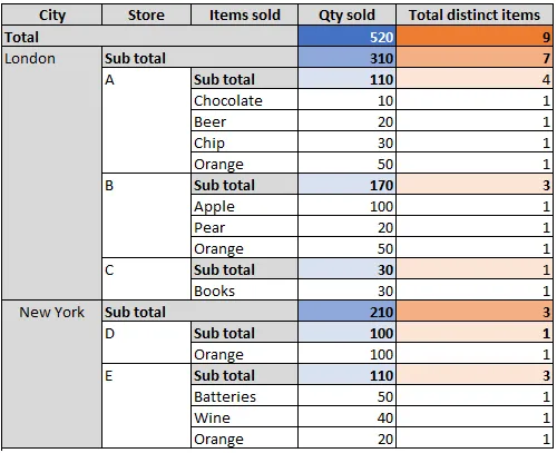
Looking at the system from the bird-eye view means aggregating many contributing factors into summary measures. Oftentimes these aggregations are straightforward such as count or sum — we call them additive aggregations, but in certain cases aggregations are complex and things just don’t add up easily. In this case, we say aggregations are non-additive. The number of distinct items purchased in retail stores is a good example of a non-additive measure: when you break it down, say, by store name or by the city — the top-level value will not be equal to the sum of contributors.

Explaining non-additive measures: parent and siblings aggregations
Calculating non-linear aggregations is often an expensive and hard task, but what is even harder is to be able to dynamically explore and explain how this aggregation is driven by underlying contributors.
This problem is called contribution analysis. A typical example would be:
- Allocating firm-wide economic capital down to trading desks,
- Line-by-line surplus requirements for insurance companies,
- Dynamic resource allocation.

In this post we will see how “parent” and “sibling” data relationships in Atoti allow you to easily navigate any hierarchy of data and implement your on-the-fly allocation rules.
I will be showing you different ways to explain non-additive measures against financial examples, as the calculations are often non-additive — think about Value-at-Risk, FRTB, EAD and others.
Solution #1: Allocating a non-additive measure into additive components
In finance, the firm-level risk measure needs to be attributed down to desks in an additive manner to identify top risk drivers and allocate costs. Firm-level capital measure is non-additive, or more specifically it is sub-additive:

We can implement a measure allocating capital into additive components, formally the desired behaviour can be described with this formula:

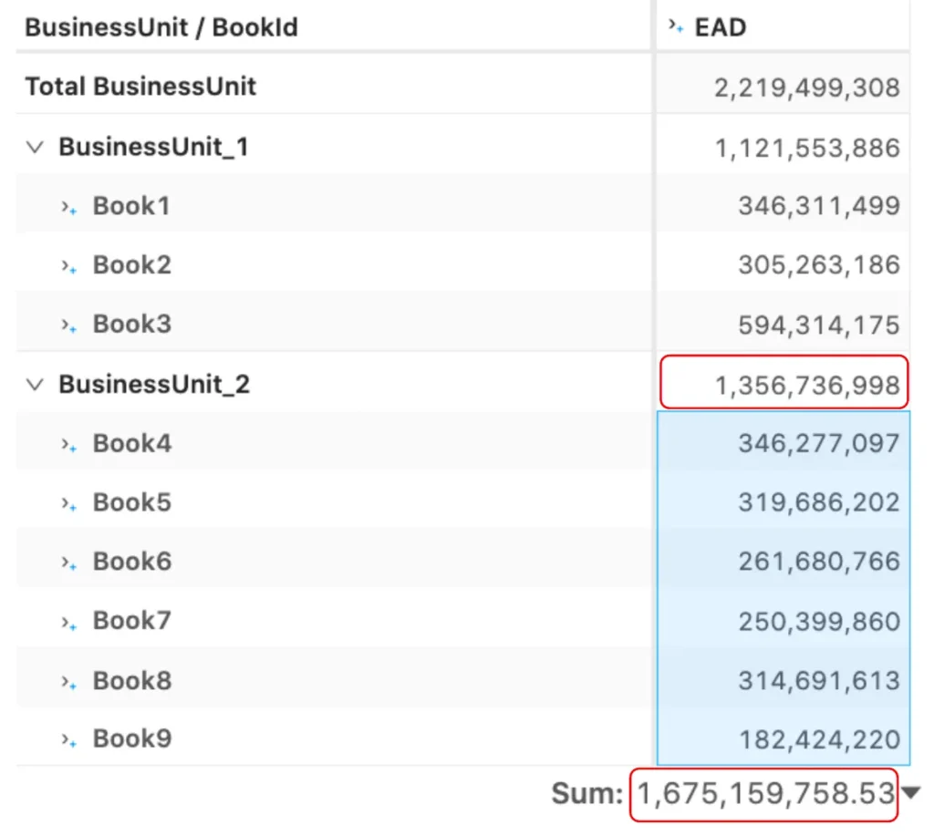
For example, the “Exposure-at-Default” (EAD) risk measure implemented in the SA-CCR notebook in the Atoti gallery is a non-linear measure, i.e. if I break down the firm-level EAD, say, by a “book” — the sum of contributors will not be equal to the EAD calculated across “all books”. See, for instance, that EAD for the BusinessUnit_2 is 1,356 Mio vs the sum of EAD for the contributing books is 1,675 Mio.

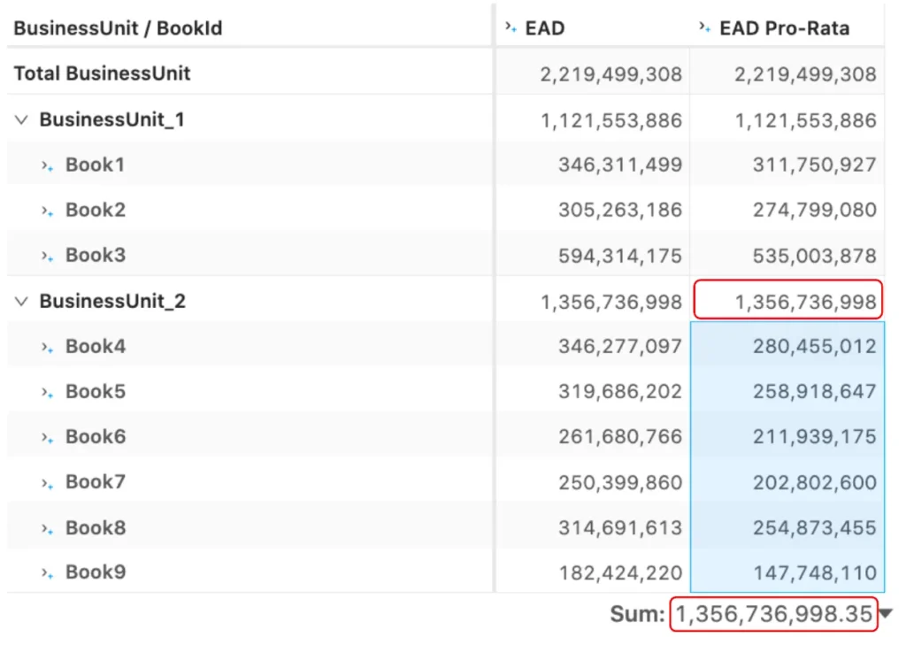
I need to implement an allocation methodology to make EAD behave “additively”: so that the sum of book level calculations match the firm-level number, as in the following screenshot for the “EAD Pro-Rata” where the sum of the highlighted books 1,356 Mio is equal to the EAD computed across those books:

The allocation principle is a matter of a practitioner’s choice — see for
instance, “Honour your contribution” by U. Koyluoglu and J. Stoker
published in www.RISK.net in April 2002 or Capital Allocation to Business Units and Sub-Portfolios: the Euler Principle by D. Tasche.
In this post let’s take a simple example — pro-rata allocation — to illustrate the parent/child/sibling Atoti concept.
To implement an allocation for a measure, I will multiply the value calculated above the contributor — at the parent level — by the weight of that contributor.

Let’s compute the weight as a ratio of a book’s EAD by the sum of standalone calculations:

This is a simple way to scale the sum of elements back to the allocated value. As I mentioned earlier, the allocation principle can be more sophisticated to satisfy the desired properties. We’ll explore one more example — Euler allocations — in one of the next posts.
To implement the “EAD Pro-rata”, I first defined a measure which computes the sum of EADs for each of the book’s “siblings” including the current book itself (denoted as f(X)+f(Y) above):
m["EAD_sum_by_book"] = tt.agg.sum(m["EAD"], scope=tt.scope.siblings(h["BookId"]))Then the weight w for each book can be defined as:
m["Book_weight"] = m["EAD"] / m["EAD_sum_by_book"]I will be using Atoti’s parent_value function to retrieve the value above my current contributor (above current book) — you may read more about the parent_value function in the Atoti doc:
m["EAD_across_books"] = tt.parent_value(
    m["EAD"], h["BookId"], degree=1, total_value=m["EAD"], apply_filters=True
)
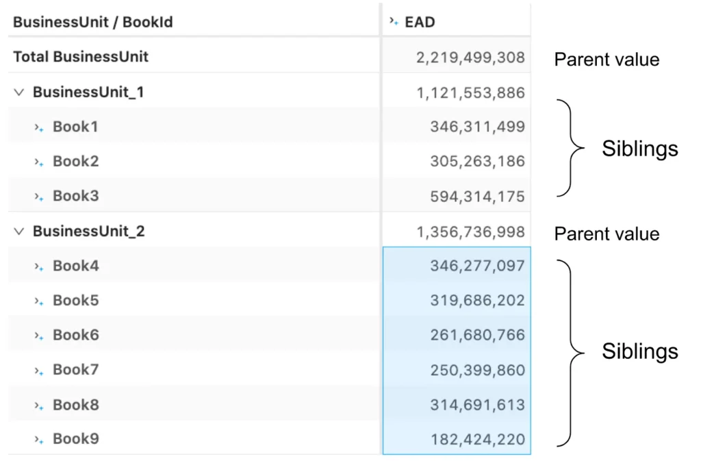
As a recap of the above, this screenshot is showing what are the parent values and what are the siblings:

Finally the Pro-Rata measure is a simple product:
m["EAD Pro-Rata"] = m["Book_weight"] * m["EAD_across_books"]If a hierarchy has multiple levels — for example, as in a banks’ organizational hierarchy — the allocation of the top-level values can apply recursively every time the user expands it.
Conclusion
In this post, we discussed how to use parent and sibling relationships in Atoti to implement contributory measures and explained non-additive measures. I hope the described techniques can help you build powerful analytic applications!


